Scaling Laws: Kaplan, Chinchilla, and Why Nobody Trains Chinchilla-Optimal
- Lakshmanan LN
- Machine learning , Deep learning , Llms
- May 5, 2026
Table of Contents
Say you’ve got loss numbers from a 40M-parameter run and a 400M-parameter run, same data, same architecture family, same optimizer. Someone asks: how well will a 70B-parameter version do, and how much data should it see? Answering that by training the 70B model first means committing seven or eight figures of compute before you know whether it was worth it.
Neural scaling laws are the reason labs mostly don’t have to do that. Across a wide range of scales, a language model’s test loss — plain cross-entropy, next-token prediction — turns out to be a remarkably well-behaved function of three numbers: parameter count, training tokens, and total compute. Well-behaved enough that a handful of cheap, small-scale runs let you extrapolate to models you haven’t built yet. That predictive power — not the banal “bigger models are better” — is the actual finding, and it turned “how big a model should we build” from a guess into a forecasting problem with error bars.
This post covers what that power law actually says; why OpenAI’s Kaplan et al. (2020) and DeepMind’s Hoffmann et al. (2022, “Chinchilla”) looked at the same allocation question and reached different conclusions about how to spend a training budget; why that disagreement had a mostly mundane explanation; and why, once you account for inference cost, almost nobody trains the model either paper’s optimum recommends.
The claim, precisely
Strip away the history and the claim is three power laws, one per axis, each valid when the other two aren’t the bottleneck:
L(N) = (N_c / N)^α_N     loss vs. parameters, data and compute held ample
L(D) = (D_c / D)^α_D     loss vs. training tokens, model size held ample
L(C) = (C_c / C)^α_C     loss vs. compute, N and D both allocated optimally
N_c, D_c, C_c and the α’s are fitted constants with no physical meaning beyond “where this curve crosses these axes.” The content is in the shape: a power law y = a·x^(-b) is a straight line when you plot log(y) against log(x), with slope -b. Plot loss against parameter count on log-log axes, see the points fall on a line, and you’ve measured α_N as that slope — and, crucially, you can keep following that line out to parameter counts you haven’t trained yet.
Here’s the fitting procedure, on synthetic numbers standing in for a real small-scale sweep (illustrative, not actual Kaplan et al. data — the point is the mechanics):
import numpy as np

# (N, loss) pairs from a handful of runs, everything else held fixed
N = np.array([1e6, 1e7, 1e8, 1e9])
L = np.array([4.9, 3.9, 3.3, 2.8])          # nats/token, illustrative

log_N, log_L = np.log(N), np.log(L)
slope, intercept = np.polyfit(log_N, log_L, 1)   # best-fit line in log-log space

alpha_N = -slope
N_c = np.exp(intercept / alpha_N)
print(f"alpha_N ~ {alpha_N:.3f}, N_c ~ {N_c:.2e}")

N_big = 7e10                                  # a 70B-param model we haven't trained
L_pred = (N_c / N_big) ** alpha_N
print(f"predicted loss at N={N_big:.0e}: {L_pred:.3f}")
Plotted, that’s the whole argument in one picture — the four runs land on a line, and the line keeps going:
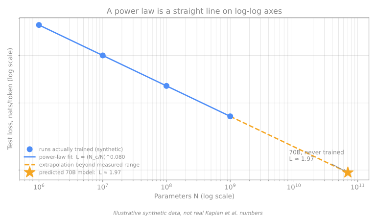
Four runs, a polyfit call, and a prediction about a model 70x bigger than anything actually trained. Everything else in this post is about getting the details of that extrapolation right — what “optimal allocation” means, and where the trick stops working.
Why this held up, and where it stops
The surprise wasn’t that bigger models do better — everyone training neural nets already believed that. It’s that despite training being a noisy, non-convex mess where individual runs are unpredictable, the aggregate loss-vs-scale relationship is smooth: Kaplan et al. report the trend holding over more than seven orders of magnitude, and largely indifferent to architecture. Width, depth, number of heads have, in their words, “minimal effects” on the loss a model of a given parameter count achieves, as long as the shape isn’t pathological. That’s what makes a small sweep informative about scale in general rather than about your specific choice of knobs.
Taken literally, though, a bare power law implies loss keeps falling toward zero as N, D, or C go to infinity — which can’t be right, since natural text has genuine entropy no model can predict away. Both papers’ complete functional forms build in a floor. Kaplan et al. couple N and D multiplicatively:
L(N, D) = [ (N_c/N)^(α_N/α_D) + D_c/D ]^α_D
Hoffmann et al. split the floor out as an explicit additive term:
L(N, D) = E + A/N^α + B/D^β
with fitted E ≈ 1.69, A ≈ 406.4, α ≈ 0.34, B ≈ 410.7, β ≈ 0.28. E is read directly as an estimate of the entropy of natural text: the loss of a model that has fully learned the statistics of language but still can’t predict genuinely unpredictable tokens. A/N^α and B/D^β are the reducible part — what more parameters or more tokens still buy you — decaying toward E, not through it.
The one piece of arithmetic worth memorizing: C ≈ 6ND
Everything downstream — the entire “how do I split compute” question — depends on converting between model size, data size, and compute. The conversion is approximate but good, and it’s the one number in this whole area you can check yourself against a model you already know.
A forward pass costs roughly 2N FLOPs per token — each parameter is touched by about one multiply-add as an activation flows through it. The backward pass costs about twice that, ~4N FLOPs per token, since gradients flow through the same matrix multiplies twice (once for inputs, once for weights). Forward plus backward: ~6N FLOPs/token, so training on D tokens costs
C ≈ 6 · N · D
Check it against a model whose numbers you already know:
N, D = 175e9, 300e9     # GPT-3: parameters, training tokens
C = 6 * N * D
print(f"{C:.2e} FLOPs")  # ~3.15e23 FLOPs
That’s the figure you’ll see quoted for GPT-3’s training compute, built from nothing but N, D, and a factor of 6.
One convention worth keeping straight: N here is Kaplan et al.’s non-embedding parameter count — they found embedding/unembedding matrices behave differently, distorting the fit at small scale where the embedding table is a bigger fraction of the total. Check which convention a “parameter count” is using before comparing numbers across papers. And C ≈ 6ND is what makes IsoFLOP profiling (next section) mechanically simple: fix C, pick any N, and D = C/(6N) falls out for free.
Splitting the budget: Kaplan’s answer
Given a fixed compute budget, how should you split it between N and D? Kaplan et al. fit their laws and solved for the loss-minimizing allocation:
N ∝ C^0.73 B (batch size) ∝ C^0.24 S (steps) ∝ C^0.03 (D = B · S)
Model size should grow much faster than data — roughly N^0.73 against a data budget growing more like C^0.27. Equivalently, D ∝ N^(α_N/α_D) ≈ N^0.74: their own gloss is that an 8x bigger model “only” needs about 5x more data (8^0.74 ≈ 4.7). Their headline conclusion, stated directly in the abstract: “optimally compute-efficient training involves training very large models on a relatively modest amount of data and stopping significantly before convergence.”
That sentence is close to a design spec for GPT-3: 175B parameters, trained on roughly 300B tokens — a large model, stopped well short of convergence, by design, because the scaling law said that was compute-efficient.
Chinchilla re-runs the experiment, three ways
Two years later, Hoffmann et al. asked the same allocation question with a more careful design. Where Kaplan et al. leaned mainly on one method, Hoffmann et al. triangulated across three independent approaches and checked that they agreed:
- Fix model size, vary tokens. Train the same sizes (70M-10B params) at several token budgets and read off, per size, the loss-minimizing token count.
- IsoFLOP profiles — their signature technique, walked through below.
- Parametric fit. Fit L(N,D) = E + A/N^α + B/D^β to every final loss from approaches 1 and 2 at once, then solve analytically for N_opt(C), D_opt(C).
IsoFLOP profiling is worth walking through step by step — it’s simple enough to redo at small scale, and it’s the intuition underneath the other two approaches. The problem it solves: train models at whatever size and data you like, and you can’t tell whether a bigger model won because it’s bigger or because it happened to see more data. IsoFLOP profiling controls for that by holding compute fixed and letting size and data trade off inside that fixed budget:
    flowchart TD
	    A["Pick a fixed compute budget C_i<br/>e.g. 1e21 FLOPs"] --> B["Sweep model sizes N,<br/>small to large"]
	    B --> C["For each N, solve D = C_i / (6N)<br/>so every run costs exactly C_i"]
	    C --> D["Train each (N, D) pair to completion"]
	    D --> E["Plot final loss vs. log(N)"]
	    E --> F["Fit a parabola;<br/>read off its minimum: N_opt(C_i)"]
	    F --> G{"More compute<br/>budgets to test?"}
	    G -->|yes| A
	    G -->|no| H["Fit a power law through all<br/>(C_i, N_opt) points: N_opt ∝ C^a"]
Hoffmann et al. ran this at 9 compute budgets from 6×10^18 to 3×10^21 FLOPs, training over 400 models (~70M to ~16B params, 5B to 500B tokens) to trace out N_opt(C). One IsoFLOP slice, in code, is just C ≈ 6ND run in reverse:
C_i = 1e21   # one IsoFLOP slice, FLOPs
for N in [1e8, 3e8, 1e9, 3e9, 1e10]:
    D = C_i / (6 * N)
    print(f"N={N:.1e} params -> D={D:.2e} tokens, same {C_i:.0e} FLOPs")
Every row costs the same compute; only the split between size and data changes. Train all of them, plot loss against N, fit a parabola, and the vertex is the answer for that slice of compute.
The verdict: scale N and D about equally
All three approaches landed in roughly the same place — three different ways of asking the question, converging on the same answer:
| Approach | N_opt ∝ C^a | D_opt ∝ C^b |
|---|---|---|
| 1. Fixed model sizes | a ≈ 0.50 | b ≈ 0.50 |
| 2. IsoFLOP profiles | a ≈ 0.49 | b ≈ 0.51 |
| 3. Parametric fit | a ≈ 0.46 | b ≈ 0.54 |
| Kaplan et al., for comparison | a ≈ 0.73 | b ≈ 0.27 |
Kaplan et al.: grow the model much faster than the data. Hoffmann et al.: grow them at roughly the same rate. Not a small disagreement — it changes the compute-optimal allocation at GPT-3-ish scale enormously.
    flowchart TD
	    C0["Fixed training compute budget C"] --> K["Kaplan et al., 2020<br/>N ∝ C^0.73, D ∝ C^0.27"]
	    C0 --> H0["Hoffmann et al., 2022<br/>N ∝ C^0.50, D ∝ C^0.50"]
	    K --> K2["Large model, comparatively little data<br/>e.g. GPT-3: 175B params / 300B tokens"]
	    H0 --> H2["Model and data grow together<br/>e.g. Chinchilla: 70B params / 1.4T tokens"]
Hoffmann et al. didn’t stop at a different exponent — they built the model their own math recommended and let it compete. Chinchilla: 70B parameters, 1.4T training tokens, trained on (by the paper’s own account) roughly the same compute budget as DeepMind’s own Gopher (280B parameters, ~300B tokens). Despite being a quarter of Gopher’s size, Chinchilla beat Gopher, GPT-3 (175B), Jurassic-1 (178B), and Megatron-Turing NLG (530B) across a wide range of downstream evaluations — including 67.5% on MMLU, more than 7 points over Gopher. A 4x-smaller model, same training compute, better benchmark: parameter count is a poor proxy for capability if the model is undertrained relative to the compute that went into it. The paper’s own diagnosis: Gopher, GPT-3, and MT-NLG had all held training tokens near ~300B while scaling parameters up, which — given the equal-scaling result — is compute-inefficient: “current large language models are significantly undertrained, a consequence of the recent focus on scaling language models whilst keeping the amount of training data constant.”
The “~20 tokens per parameter” figure you’ll see everywhere is worth being precise about: it doesn’t appear verbatim in the paper, it’s a derived rule of thumb. 1.4T / 70B is exactly 20, and the paper’s own compute-optimal frontier table clusters around that ratio across a wide range of budgets — roughly 20.0 at 400M parameters, ~20.5 at 10B, drifting up to ~22.4 by 67B. Fair summary, not a flat constant: treat it as the right order of magnitude for that regime, not a law.
Where that ~0.5 exponent actually comes from
Worth seeing the parametric fit produce that exponent rather than taking it on faith. Substitute the compute constraint D = C/(6N) into Hoffmann et al.’s functional form to collapse it to a function of N alone, then minimize:
L(N) = E + A·N^(-α) + B·(C/6N)^(-β) = E + A·N^(-α) + B·6^β·C^(-β)·N^β

dL/dN = -α·A·N^(-α-1) + β·B·6^β·C^(-β)·N^(β-1) = 0

=>  N_opt(C) ∝ C^(β / (α+β))
Plug in α ≈ 0.34, β ≈ 0.28: β/(α+β) = 0.28/0.62 ≈ 0.45, matching the a ≈ 0.46 reported for approach 3 (and by the same algebra, D_opt(C) ∝ C^(α/(α+β)) ≈ C^0.55, matching b ≈ 0.54). “Scale N and D equally” isn’t a separate empirical observation — it falls straight out of calculus once fitted α and β happen to be close to each other. Had they come out very different, equal scaling wouldn’t hold, even with the identical functional form.
So was Kaplan just wrong?
The easy version — “Chinchilla proved Kaplan et al. wrong” — gets repeated constantly and isn’t quite fair. Porian et al. (“Resolving Discrepancies in Compute-Optimal Scaling of Language Models,” 2024, NeurIPS Spotlight) reproduced Kaplan et al.’s original setup and traced most of the gap to specific, fixable choices: how last-layer/embedding parameters were counted into the compute budget, warmup-duration differences, and optimizer tuning that doesn’t transfer across scale — AdamW’s β₂ specifically needs retuning at the small batch sizes Kaplan et al.’s smaller runs used. Correct for those and the reproduction lands in “excellent agreement” with Chinchilla’s scaling law. One nuance worth keeping: careful learning-rate decay matters for absolute loss but, per Porian et al., isn’t strictly essential to the validity of the scaling-law fit itself — more specific, and more defensible, than the common shorthand “Kaplan was wrong because of the LR schedule.” Net: two studies with different, under-specified experimental controls produced different quantitative fits to the same qualitative phenomenon — not a conceptual error in the power-law framing. (A second, similarly-scoped paper, arXiv:2406.12907, covers related ground; treated here as corroborating color, checked only at the abstract level.)
Pair that with an even less-repeated nuance: Chinchilla’s own approach-3 parametric fit had a bug. Epoch AI, reproducing it from data reconstructed off the paper’s plots, found the published fit matched their reconstruction poorly, reported implausibly narrow confidence intervals, and was internally inconsistent with the paper’s own approaches 1 and 2 — traced to the original optimizer stopping short of full convergence and rounding of published coefficients against the underlying LaTeX source. Their corrected fit, L(N,D) = 1.8172 + 482.01/N^0.3478 + 2085.43/D^0.3658, lines up with approaches 1 and 2 — and the qualitative conclusion survives untouched. Even the paper usually cited as “fixing” Kaplan et al. had a bug in one of its own three methods, and fixing it didn’t move the headline.
Compute-optimal answers a narrower question than you’d think
Worth being pedantic about the definition, because it gets used more loosely than it supports. Chinchilla-optimal means: the (N, D) pair that minimizes training loss for a fixed training-FLOPs budget. Nothing about inference cost, latency, memory, or what the model costs once it’s answering real traffic.
LLaMA’s paper says this outright: “this objective disregards the inference budget, which becomes critical when serving a language model at scale,” and “although it may be cheaper to train a large model to reach a certain level of performance, a smaller one trained longer will ultimately be cheaper at inference.” Their comparison: “Hoffmann et al. (2022) recommends training a 10B model on 200B tokens, we find that the performance of a 7B model continues to improve even after 1T tokens.” LLaMA-1’s actual budgets: 7B and 13B on 1.0T tokens, 33B and 65B on 1.4T tokens — well past what a strict Chinchilla split would give those sizes.
Llama 3 goes further, and says so explicitly: “While the Chinchilla-optimal amount of training compute for an 8B parameter model corresponds to ~200B tokens, we found that model performance continues to improve even after the model is trained on two orders of magnitude more data. Both our 8B and 70B parameter models continued to improve log-linearly after we trained them on up to 15T tokens.” 15T tokens against 8B parameters is roughly 1,875 tokens per parameter — about 75x the ~20:1 Chinchilla ratio — and loss was, by Meta’s own account, still improving log-linearly when they stopped.
    flowchart LR
	    A["Training compute budget C"] --> B["Chinchilla-optimal (N*, D*)<br/>minimizes training loss only"]
	    B --> C{"Expected inference volume<br/>over the model's deployed life?"}
	    C -->|modest| D["Train near (N*, D*)"]
	    C -->|"large: billions of requests"| E["Shrink N below N*,<br/>push D well above D*<br/>= 'overtraining'"]
	    E --> F["Higher training cost,<br/>cheaper cost per token served"]
Not a failure to read the paper — it’s deliberate. Sardana et al., “Beyond Chinchilla-Optimal: Accounting for Inference in Language Model Scaling Laws,” extend the same methodology to jointly minimize training and inference compute given an assumed request volume, instead of training compute alone. Their framing: “LLM researchers expecting reasonably large inference demand (~1B requests) should train models smaller and longer than Chinchilla-optimal.” Across 47 trained models, quality kept improving out to token-per-parameter ratios as extreme as ~10,000 in some regimes — while fits calibrated only on “typical” near-20:1 ratios tend to overestimate loss out there, meaning naive extrapolation of the original Chinchilla fit that far outside its measured range is itself unreliable.
Napkin math: why overtrain at all
The intuition for why a smaller, longer-trained model wins isn’t spelled out directly in any of these papers, but it falls out of arithmetic already on the table, so it’s worth doing explicitly.
Training compute for a roughly Chinchilla-shaped model, using ~20 tokens/parameter as a stand-in: C_train ≈ 6·N·(20N) = 120·N². Inference is forward-pass only, so serving D_inf tokens costs roughly C_inf ≈ 2·N·D_inf. Set them equal to find the crossover — the point where you’ve spent as much compute serving the model as you spent training it:
2·N·D_inf = 120·N²
D_inf = 60·N
Once you’ve served on the order of 60 tokens per parameter — the same order of magnitude as the training tokens themselves — inference compute has caught up with training compute. For a 70B model that’s roughly 4.2 trillion served tokens, which a popular API can plausibly burn through in weeks, not years. Every token served after that point is compute spent on top of an already-recouped training cost, for the entire life of the deployment. That’s the real argument for shrinking N and growing D past Chinchilla-optimal: training compute is a one-time cost, inference compute is recurring and, for anything popular, eventually dwarfs it.
Trade-offs and where this breaks down
Extrapolation outside the measured range isn’t guaranteed. Kaplan et al. say plainly they “do not have a solid theoretical understanding for any of [the] proposed scaling laws,” and flag their own D-scaling behavior as “mysterious” at very large model size, with an apparent breakdown of the simple picture around C* ~ 10^4 PF-days. Hoffmann et al. had only two genuinely large-scale runs — Chinchilla and Gopher — to validate against at the top of their range, and note some concavity in log(N_opt) at high compute relative to what a clean power law predicts. Treat the fitted exponents as locally accurate over the measured range, not as physical constants.
The 20:1 ratio is a regime, not a constant — and “N” isn’t even defined the same way everywhere. It’s specific to Hoffmann et al.’s dataset, tokenizer, and architecture family, over a compute range up to roughly 10^24 FLOPs, and it drifts within their own results (creeping from ~20 toward ~22 as compute scales up). It also assumes enough unique high-quality tokens exist; data-constrained regimes (Muennighoff et al. — flagged here only as a pointer, not independently verified in writing this) shift the picture once you’re forced to repeat data. Separately, “N” means non-embedding parameters in Kaplan et al.’s convention and closer to total parameters elsewhere, and “a token” is whatever a given paper’s tokenizer produces — numbers across papers and technical reports don’t line up cell-for-cell without checking conventions first.
Loss scaling smoothly isn’t the same claim as capability scaling smoothly. Everything above describes cross-entropy loss, which is smooth by construction. Downstream benchmarks can look discontinuous or “emergent” with scale, but Schaeffer et al. (“Are Emergent Abilities of Large Language Models a Mirage?”, NeurIPS 2023) argue much of that is an artifact of nonlinear, discontinuous metrics like exact-match accuracy — swap to a continuous metric on the same model outputs and the discontinuity often shrinks or disappears. This is a genuinely contested area of the literature, not a settled rebuttal.
Even the reference fits have needed correcting. Chinchilla’s own parametric fit had a bug that Epoch AI’s replication caught, as above — good reason to hold any single quoted coefficient (E, A, α, B, β, or Kaplan’s N_c, D_c) a little loosely rather than as ground truth to the last significant figure.
Some of the inference-side numbers in this post are secondary-sourced. Sardana et al.’s own claims — smaller-and-longer for high inference demand, 47 models trained, quality improving out to ~10,000 tokens/parameter in some regimes — are solid, checked directly against the paper’s own framing. A specific figure sometimes quoted alongside this work — a Chinchilla-style 70B model “only 1% off compute-optimal but costing 36% more than a cost-optimal model” under a 2-trillion-token inference scenario — comes from a secondary engineering-blog summary rather than the primary paper, and should be read as an illustrative estimate rather than a precise, citable number.
The practical upshot
Setting a real training budget today follows roughly this sequence: pick a compute budget C, use something like the IsoFLOP procedure (or borrow published α, β fits) to find the Chinchilla-optimal (N*, D*) that minimizes training loss at that C, then — separately — estimate the inference volume the model will see over its deployed life, and deliberately move off (N*, D*) toward smaller N and larger D if that volume is large. “Compute-optimal” is a well-defined starting point, not the final answer.
That last decision — how far you can shrink N while holding a quality bar, and how long you’re willing to train to get there — also fixes the shape of the model you eventually have to serve: cost per token, memory footprint, how its KV cache behaves under load. That’s where this series goes next — and it builds on how attention itself works from the first post, if you want the mechanism underneath all of this.